The roof was reflecting light like a painted wall.
The input photo was fine. So was the segmentation. The diffusion pipeline ran without errors, and the output still failed the most basic human test: does this look like the same material if I move the sun? The wall’s reflectance characteristics were bleeding across boundaries, and the roof paid for it.
Call it single-image PBR decomposition if you want. The real problem is a per-region one.
The key insight: decomposition isn’t global, materials are local
RGB‑X (a diffusion-based decomposition pipeline) can produce the maps I need, albedo, normal, roughness, irradiance, from a single photo. The research side is in good shape.
The engineering side is the one that actually matters in a construction visualization workflow. A phone photo is a collage of different materials, and a global pass happily blends them.
Decompose the full frame and you’re asking the model to explain everything at once. Which gets you:
- “wall roughness” influencing “roof roughness”
- lighting estimates that smear across high-contrast boundaries
- normals that look plausible in isolation but don’t respect region edges
So I made a hard rule: I only decompose a region in isolation.
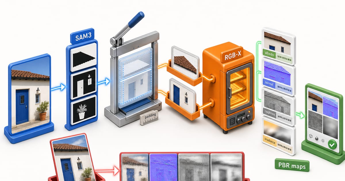
The pipeline that falls out of that rule:
- segment the photo into architectural regions (walls, roof, trim)
- crop each region with padding
- resize to satisfy the U‑Net constraint (multiples of 8)
- run RGB‑X once per channel, per region
- return per-region PBR maps to drive interactive rendering
My one analogy for this: running RGB‑X on a whole house photo is like trying to match paint by sampling the entire room, walls and ceiling and couch and floor, then wondering why the “average color” looks wrong on the trim.
How it works under the hood
Two nested passes are the ones that matter:
- a pass over regions (per SAM3 mask)
- a pass over channels (per PBR map)
And two unglamorous constraints decide whether the whole thing feels production-grade:
- padding to survive mask edge artifacts
- resizing to keep the diffusion U‑Net happy
Here’s the full data flow.
Channel-specific prompts: I don’t let the model guess what I want
RGB‑X is driven by a prompt per channel. I keep that mapping explicit and dull, because the worst failure mode is “it returned something that looks like a map.”
CHANNEL_PROMPTS = {
    "albedo": "Albedo (diffuse basecolor)",
    "normal": "Normal",
    "roughness": "Roughness",
    "irradiance": "Irradiance (estimate lighting)",
}
Nothing clever there. It’s declarative, and that’s the point: when a map looks off, I can reason about exactly which pass produced it.
One inference pass per channel (and a weird nested-list unwrap)
Each channel is a separate diffusion inference call. Expensive. It buys controllability and clarity.
The non-obvious footgun I had to handle: RGB‑X sometimes wraps the image output in an extra list, so I unwrap it before encoding.
prompt = CHANNEL_PROMPTS.get(channel)
result = rgbx_pipe(prompt=prompt, photo=photo, num_inference_steps=steps, height=h, width=w)
img = result.images[0]
if isinstance(img, list) and len(img) > 0:
    img = img[0]  # Unwrap nested list (RGB-X wraps each channel in an extra list)
if isinstance(img, np.ndarray):
    if img.max() <= 1.0:
        img = (img * 255).astype(np.uint8)
    return Image.fromarray(img.astype(np.uint8))
return img
Tiny unwrap, real consequence. Without it you can end up encoding the wrong object shape and not notice until the viewer renders garbage.
Per-region decomposition: crop first, then decompose
The region pipeline starts by decoding the photo and preparing an output array.
photo = _decode_image(request.image_base64)
img_w, img_h = photo.size
regions_out = []
I keep img_w, img_h around for one reason: every bounding-box operation needs to clamp to the original image bounds. Region pipelines that don’t clamp eventually crash on edge cases, or worse, “work” by producing misaligned crops.
Iterating masks and normalizing bbox formats
SAM3 bbox data can arrive in more than one format, so I normalize both forms before anything else touches them.
with torch.no_grad():
    for i, mask_info in enumerate(request.masks):
        bbox = mask_info.get("bbox", {})
        label = mask_info.get("label", f"region_{i}")

        # Handle both [x,y,w,h] (SAM3) and {x,y,width,height} formats
        if isinstance(bbox, (list, tuple)) and len(bbox) >= 4:
            bx, by, bw, bh = int(bbox[0]), int(bbox[1]), int(bbox[2]), int(bbox[3])
        elif isinstance(bbox, dict):
            bx, by, bw, bh = int(bbox.get("x",0)), int(bbox.get("y",0)), int(bbox.get("width",img_w)), int(bbox.get("height",img_h))
Bbox format inconsistencies are the kind of “integration tax” that never shows up in model demos. Normalize late and you end up debugging downstream artifacts that are really just coordinate parsing bugs.
The 10% padding rule (because masks are never perfect)
Even good segmentation leaves messy edges. Anti-aliasing, partial coverage, thin structures... they all conspire to produce boundary artifacts.
So I pad the crop by 10% of the bbox size.
# 10% padding
pad_x, pad_y = int(bw * 0.1), int(bh * 0.1)
x0, y0 = max(0, bx - pad_x), max(0, by - pad_y)
x1, y1 = min(img_w, bx + bw + pad_x), min(img_h, by + bh + pad_y)
Padding feels too simple to matter until you put the before and after side by side. The model gets a little context around the boundary, and the maps stop looking like they were cut out with dull scissors.
Cropping + resizing for inference
After padding and clamping, I crop the region and resize it for inference.
crop = photo.crop((x0, y0, x1, y1))
crop_resized, _ = _resize_for_inference(crop, request.target_size)
cw, ch = crop_resized.size
The resize isn’t the interesting part. The constraint it enforces is.
The U‑Net constraint: dimensions must be multiples of 8
Diffusion pipelines built on a U‑Net architecture tend to have stride and downsample constraints. In this pipeline, I enforce “multiple of 8” sizing.
def _resize_for_inference(img, target_size):
    w, h = img.size
    scale = target_size / max(w, h) if max(w, h) > target_size else 1.0
    new_w = max(8, (int(w * scale) // 8) * 8)
    new_h = max(8, (int(h * scale) // 8) * 8)
    return img.resize((new_w, new_h), Image.LANCZOS), scale
Two things are doing real work there:
- I scale down only if the region is larger than
target_size. - I quantize dimensions to multiples of 8, with a floor of 8.
I treat this as a hard requirement rather than a suggestion. Violate it and you don’t always get a clean error. Sometimes you get subtly wrong outputs, or a shape mismatch buried deep in the stack.
Running decomposition per region, per channel
Once I have a clean crop, I run all requested channels and base64-encode the results.
region_maps = {}
for channel in channels:
    channel_img = _run_rgbx_channel(crop_resized, channel, request.num_inference_steps, ch, cw)
    region_maps[f"{channel}_base64"] = _encode_image(channel_img)
The unglamorous but correct part: I pass ch, cw explicitly into _run_rgbx_channel. I don’t trust implicit resizing inside the model call, because it makes it harder to reason about what resolution each map was actually produced at.
Reliability engineering: endpoints still register when a model fails
GPU servers fail in annoying ways: missing wheels, mismatched CUDA builds, dependency regressions. When that happens I still want the server to start and expose its API surface, even if a feature is temporarily unavailable.
So I load RGB‑X conditionally and register stub request models so the endpoint can exist.
RGBX_IMPORT_OK = False
class PBREstimateRequest(BaseModel):  # Stub so endpoint registers
    image_base64: str
    channels: List[str] = ["albedo", "normal", "roughness"]
async def estimate_pbr(request):
    raise ValueError("RGB-X pipeline not available")
What that pattern really controls is where the failure lands. If RGB‑X isn’t there, it fails loudly at call time instead of failing mysteriously at boot.
Patch for Transformers constant removals
RGB‑X depends on constants that aren’t present in newer transformers.utils. I patch them in-place before import paths explode.
import transformers.utils as _tu
if not hasattr(_tu, "FLAX_WEIGHTS_NAME"):
    _tu.FLAX_WEIGHTS_NAME = "flax_model.msgpack"
if not hasattr(_tu, "ONNX_WEIGHTS_NAME"):
    _tu.ONNX_WEIGHTS_NAME = "model.onnx"
I’m not romantic about this kind of patching. It’s a pragmatic keep-the-server-alive move, and the win is operational: the rest of the pipeline can still run, and the failure mode is constrained.
The procedural PBR fallback: the viewer always works
Even with a solid GPU pipeline, I don’t want the 3D experience to depend on it. If decomposition is unavailable, I still want materials that respond to light in a plausible way.
So on the client side I generate textures procedurally, using FBM noise and a height-to-normal conversion.
FBM noise: cheap structure that reads like material
function fbmNoise(x: number, y: number, octaves = 4, seed = 0): number {
  let value = 0, amplitude = 0.5, frequency = 1, maxValue = 0;
  for (let i = 0; i < octaves; i++) {
    value += amplitude * smoothNoise(x * frequency, y * frequency, seed + i * 100);
    maxValue += amplitude;
    amplitude *= 0.5;
    frequency *= 2;
  }
  return value / maxValue;
}
The detail that matters is the amplitude and frequency schedule: halve amplitude, double frequency. Simplest way I know to get multi-scale texture without shipping image assets.
Height → normal: turning scalar bumps into lighting response
function heightToNormal(heightData: Uint8Array, width: number, height: number, strength = 1.0): Uint8Array {
  const normalData = new Uint8Array(width * height * 4);
  for (let y = 0; y < height; y++) {
    for (let x = 0; x < width; x++) {
      const idx = (y * width + x) * 4;
      const left = heightData[y * width + Math.max(0, x - 1)] / 255;
      const right = heightData[y * width + Math.min(width - 1, x + 1)] / 255;
      const up = heightData[Math.max(0, y - 1) * width + x] / 255;
      const down = heightData[Math.min(height - 1, y + 1) * width + x] / 255;
      const dx = (left - right) * strength;
      const dy = (up - down) * strength;
      const dz = 1.0;
      const len = Math.sqrt(dx * dx + dy * dy + dz * dz);
      normalData[idx] = Math.floor((dx / len * 0.5 + 0.5) * 255);
      normalData[idx + 1] = Math.floor((dy / len * 0.5 + 0.5) * 255);
      normalData[idx + 2] = Math.floor((dz / len * 0.5 + 0.5) * 255);
      normalData[idx + 3] = 255;
    }
  }
  return normalData;
}
This is the difference between a flat sticker and something that actually reacts when you move the light. Even as a fallback, it preserves the core promise: materials look different under different illumination.
Nuances that matter in practice
A per-region diffusion pipeline sounds straightforward until you feel the edges.
Why the naive “full image” approach fails
The failure isn’t that RGB‑X is bad. The objective is misaligned:
- The model is encouraged to explain the entire frame coherently.
- Coherence across the frame is not what you want when the frame contains multiple materials.
Per-region cropping forces the model into the right local context. The model didn’t get smarter. The problem got smaller.
Why padding is a real parameter, not a magic number
I use 10% padding because it’s proportional rather than absolute. Thin regions get a little context; large regions get enough boundary room to avoid edge artifacts.
The tradeoff is obvious. Too much padding and you reintroduce cross-material contamination. Too little and the crop becomes “mask-edge dominated.”
The cost tradeoff: channel passes multiply quickly
Each region runs multiple diffusion passes, one per channel. That’s computationally heavy by definition.
I accept it for what it buys, a clean mental model:
- each output map has a specific prompt
- each prompt corresponds to a single inference call
When something looks wrong, I can isolate which pass is responsible.
The operational tradeoff: patching dependencies isn’t pretty
The Transformers constant patch is not elegant. It’s a stability move.
The alternative is worse: a server that fails to start because a dependency changed a constant name. I’d rather keep the pipeline alive and constrain the failure mode.
Closing
When I stopped decomposing the whole photo and started decomposing regions, the outputs stopped looking like “AI texture soup” and started behaving like materials. Local, bounded, believable under changing light.