Model Failure Is a Time Series

A quiet model is easy to trust for the wrong reason. The failure mode that forced my hand was not a dramatic crash or an exception in the inference server. It was worse: the primary predictor could keep emitting ordinary-looking forecasts while the property I actually needed for execution — whether the next prediction would be correct enough to act on — was changing underneath it.

That is why I built CTF as a separate reliability forecaster in the Pramaana crypto research stack. Not another directional signal. Not a committee. Not a narrative layer around the model. CTF is a lightweight inference helper in inference/ctf_predictor.py that turns recent uncertainty behavior into a fixed reliability feature vector and predicts the probability that the next primary-model call deserves trust.

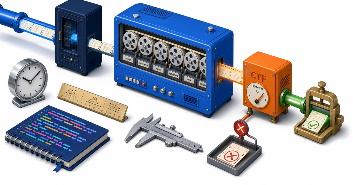
The transferable idea is the title taken literally: model failure is a time series. Reliability is not just a scalar attached to one row. If the main predictor has an uncertainty trail — entropy, confidence, calibration width, agreement, drift, recent hit rate — then trust is itself a time series. CTF exists because I wanted the execution layer to stop treating confidence as a one-frame photograph and start treating it as telemetry.

This post is not about adding yet another confidence threshold. I had already built several forms of gating, calibration, and meta-evaluation into the system: conformal intervals, per-asset calibration, cost-baked EV checks, and post-deployment filter audits. CTF is a narrower contribution. It models the evolution of uncertainty behavior as a supervised reliability target. The primary model answers, “What happens next?” CTF answers, “Is this model currently in a state where its next answer is likely to be right?”

Predict correctness, not price

The naive version of uncertainty handling is to read one confidence value and make a decision from it. High confidence means act. Low confidence means stay flat. That is clean, but it is too shallow for a regime-shifting market.

A single uncertainty snapshot tells me how the model feels about the current input. It does not tell me whether confidence has been deteriorating for the last hour, whether entropy has become unstable across assets, whether conformal width is expanding, whether the model has been right recently, or whether the current confidence value is abnormal relative to its own local history.

Those are not properties of one prediction. They are properties of a sequence.

CTF is built around that distinction. The primary model emits a forecast and uncertainty telemetry. CTF consumes a bounded recent-history window and predicts correctness of the next forecast. That keeps the tasks separate:

• the primary predictor models market path behavior;
• CTF models the primary predictor’s current reliability state;
• the execution layer consumes both through a cost-aware gate.

A price predictor tries to model the market. A correctness predictor models the predictor.

The analogy I keep coming back to is a racing engine. The primary model is the engine producing torque. CTF is not a second engine bolted to the hood; it is the telemetry system watching temperature, vibration, and pressure over the last few laps. You do not add telemetry because the engine never works. You add it because engines often sound fine right before they stop being fine.

Here is the shape of the layer:

The important transformation happens in the middle. The system stops asking only, “What did the model just say?” and starts asking, “How has the model been behaving?”

Why this is different from a confidence gate

A confidence gate is memoryless unless you explicitly give it memory. It takes the current output, compares it to a threshold, and either passes or blocks the trade. That can be useful, but it collapses the reliability problem into a single coordinate.

CTF is not that. CTF is a supervised model trained on windowed behavior. It can learn that the same current confidence value means different things depending on the preceding trajectory.

For example, suppose the primary predictor emits a confidence value of 0.58. A simple gate sees 0.58 and applies one rule. CTF sees the surrounding state:

• confidence was 0.74, 0.69, 0.63, then 0.58 over the last few observations;
• attention entropy has been rising;
• cross-asset dispersion has widened;
• recent correctness has fallen below the local baseline;
• conformal width is expanding for the same assets that now produce trade candidates.

That is a different situation from a stable 0.58 in a low-dispersion regime where the model has been consistently right. The current scalar is identical. The reliability state is not.

This is the novelty that matters. The model is not “more cautious” because a human wrote a more conservative if-statement. It is trained to map temporal uncertainty telemetry to a correctness probability.

That distinction also keeps CTF separate from the older XGBoost meta-filter work I ran before. The post-deployment audit of that filter was painful but useful: the apparent win-rate lift was not statistically solid, and the filter selected a fatter-tailed loss distribution. A meta-filter that passes trades based on static signal descriptors can look good in aggregate while quietly changing the tail profile of the trades it allows through.

CTF is designed around the lesson from that failure. It does not try to be a second trading strategy hidden behind a pass/fail switch. It predicts whether the primary model’s next answer is likely to be correct, using a time-indexed reliability state. That is a smaller job and a cleaner supervised target.

The supervised target: correctness at the next prediction

The target for CTF is not future return. It is not realized P&L. It is not “would this trade have made money after fees?” Those are execution outcomes, and they mix model quality with sizing, spread, slippage, funding, stops, and path-dependent order handling.

The CTF label is correctness of the primary prediction at the prediction horizon. For a directional head, that means the predicted direction matches the realized direction over the same horizon. For a path-passage formulation, it means the predicted passage event matches the realized barrier event the execution layer evaluates. The important rule is alignment: the correctness label must be defined against the same event the primary model claimed to predict.

That sounds obvious, but it is where a lot of meta-models go bad. If the primary model predicts a 60-minute direction and the reliability model is labeled against post-cost trade profitability, the meta-model is no longer measuring predictor correctness. It is measuring a mixture of predictor correctness and execution mechanics. Sometimes that is useful, but it is not CTF.

The CTF label is deliberately close to the primary model’s semantic contract:

• at time t, the primary model emits a prediction for horizon h;
• the CTF feature vector is built only from telemetry available at or before t;
• when the future outcome at t + h is known, the row receives a binary correctness label;
• that label becomes the supervised target for the reliability model.

The no-leakage rule is strict. The CTF row at time t cannot include the correctness of the prediction made at t, because that outcome is not known yet. It can include rolling correctness for earlier predictions whose horizons have already resolved. If the horizon is one hour, the most recent eligible correctness observation is from a prediction at or before t - h, not from the prediction being scored now.

That one detail is the difference between a reliability model and a disguised lookahead bug.

The history buffer is the boundary between models

A recent-history window sounds mundane until it becomes the contract between the primary predictor and the reliability predictor.

The primary model produces a stream of values: prediction, confidence, entropy, conformal width, asset, timestamp, and eventually realized correctness. CTF does not consume the raw stream as an unbounded sequence. The helper maintains a bounded buffer and compresses recent behavior into a fixed feature vector.

That compression is intentional. I did not want the execution gate to depend on variable-length sequence handling or call-time improvisation. A fixed schema makes the reliability layer testable, serializable, and comparable between training and inference.

The buffer holds only information that would have existed when a live decision was made:

• current primary-model telemetry for the candidate prediction;
• prior telemetry for the same asset or asset group;
• resolved correctness from older predictions;
• contemporaneous cross-asset uncertainty measurements;
• derived rolling statistics over the recent window.

It excludes anything that requires future knowledge:

• realized correctness of the current prediction;
• realized return over the current prediction horizon;
• post-trade P&L from a decision that has not completed;
• any feature recomputed with future rows accidentally included in a rolling window.

That last class of bug is easy to miss. Pandas rolling operations, joins between prediction logs and realized outcomes, and cross-asset aggregates can all leak if the index semantics are sloppy. The implementation discipline is to treat CTF rows exactly like live inference snapshots. If the value was not known at the timestamp being scored, it does not belong in the feature vector.

The fixed feature vector then captures several kinds of reliability evidence, each answering a separate question:

Telemetry signal	Reliability question it answers
Level	Where has uncertainty been sitting recently?
Change	How abruptly is uncertainty moving right now?
Trend	Is that movement persistent, or just noise?
Dispersion	Is the uncertainty isolated to one asset, or spreading across many?
Recent accuracy	Have resolved prior predictions actually been right?
Calibration state	Is interval width or calibrated probability shifting?
Drift	Is the current telemetry distribution departing from its recent baseline?

Means, deltas, trends, dispersion, and rolling hit rates are not decorative statistics. Each answers a separate reliability question. The level tells me whether the model is operating in a generally uncertain state. The delta tells me whether the state just changed. The trend tells me whether the change is noise or a persistent move. Dispersion tells me whether the issue is asset-local or system-wide. Rolling correctness tells me whether the model’s recent self-assessment has been earning trust.

Attention entropy is telemetry, not a verdict

In the FT-Transformer path, attention entropy is one of the most useful telemetry signals because it is closer to the model’s internal allocation of attention than a final probability alone. A final softmax collapses the whole forward pass into one number over the outputs; attention entropy instead measures how evenly the model spread its focus across input features on the way there, so it can expose the model hedging across many weak cues or fixating on a single brittle one even when the output probability looks unchanged. But I do not treat entropy as a magic score.

A single entropy value can be misleading for the same reason a single confidence value can be misleading. High entropy might mean the model is genuinely uncertain. It might also be normal for a specific asset, horizon, or volatility regime. Low entropy might mean the model has found a clean structure. It might also mean the model has collapsed onto a brittle shortcut.

The trajectory is the point. CTF watches how entropy behaves over time and relative to the local population of assets. Rising entropy across the universe is different from rising entropy in one thin asset. A sudden entropy jump after a long stable period is different from an asset whose baseline is noisy. A high-entropy state with improving resolved correctness is different from a high-entropy state with deteriorating correctness.

That is why I prefer to call these inputs telemetry rather than explanations. They are measurements from the model while it works. CTF learns which telemetry patterns have historically preceded correct or incorrect primary-model calls.

The same logic applies to conformal width. Wider intervals often mean less precise forecasts, but width by itself is not the decision. What matters is whether width is expanding, whether it is expanding faster than usual, whether it is expanding across correlated assets, and whether the model has recently remained correct under similar width dynamics.

The feature vector gives the reliability model those comparisons without turning the primary predictor into a monolith that must simultaneously forecast price, calibrate itself, diagnose drift, and decide execution.

Train/serve parity is a first-class constraint

A reliability layer can fail even when the concept is right if the training features and inference features drift apart. I had already seen this class of problem in the earlier meta-filter work, where train/serve skew around kelly_fraction was a likely contributor to bad live behavior. CTF was built with that scar tissue in mind.

The feature schema is treated as a contract. Training and inference use the same ordered feature list, the same definitions, the same window semantics, and the same missing-value policy. The CTF helper emits a fixed vector rather than a loose dictionary that downstream code can accidentally reorder.

The important pieces of the contract are:

• feature names are explicit and versioned with the model artifact;
• column order is preserved at serialization time;
• training rows are generated by replaying historical predictions as if they were live;
• inference rows are generated by the same feature builder, not a hand-written approximation;
• missing values from insufficient warm-up history are handled the same way in both paths;
• assets that lack enough resolved history are either scored conservatively or withheld until the buffer is warm.

Warm-up behavior deserves special attention. If the model needs a 32-observation window, the first few rows for an asset cannot pretend to have a full history. There are only three honest choices: do not score until the buffer is warm, use features that explicitly encode the short history length, or route the candidate through a conservative fallback. What I avoid is silently filling the window with values that make the first live rows look cleaner than they are.

Cross-asset features have their own parity trap. In training, it is tempting to compute dispersion across all rows in a timestamp bucket after the full dataset has been assembled. In live inference, only the assets scored at that time are available, and some may be missing due to exchange, ingest, or latency issues. The CTF feature builder has to make that mismatch explicit. The dispersion feature cannot depend on a perfect historical panel if live inference will see an imperfect one.

This is why I think of the history buffer as a boundary, not just a container. It enforces what the CTF model is allowed to know.

Validation before the trust probability reaches execution

A probability is useful only if it behaves like a probability. Before CTF can influence a gate, I need to know whether its scores are ordered correctly and whether their magnitudes are calibrated well enough to consume.

The first validation pass is ranking: when CTF assigns higher trust probabilities, does realized correctness actually rise? I check this by binning predictions into score buckets and comparing empirical correctness across buckets. If the model cannot rank reliability states, it has no business gating trades.

The second pass is calibration: when CTF emits 0.70, does that bucket land near 70% correctness, after accounting for sample size and regime splits? Perfect calibration is not realistic in a drifting market, but gross miscalibration is dangerous because the execution gate may treat the score as composable with expected value, risk, or size.

The third pass is regime stratification. A reliability model that only works during one volatility regime is not a reliability model; it is a regime artifact. I care about performance across realized-volatility buckets, asset tiers, time folds, and market phases. This is especially important in crypto, where a one-year window can contain calm bearish drift, violent bullish expansion, and corrective chop. A model that passes on aggregate can still fail exactly when the system most needs it.

The fourth pass is decision impact. CTF is not validated only by AUC or log loss. I also inspect what the gate would have done differently:

• which candidates would have been blocked;
• whether blocked candidates were actually lower quality;
• whether the model changes the tail of accepted losses;
• whether it reduces participation in a way that destroys opportunity;
• whether it creates asset concentration by vetoing some names more than others.

That last point came directly from the meta-filter postmortem. A filter can improve the headline win rate and still pass worse losses. For CTF, I inspect the distribution of allowed and vetoed outcomes, not only the average.

Only after those checks does the trust probability become eligible for the execution path.

The bar I hold it to in shadow mode is narrow and specific. The vetoes should cluster in exactly the windows where the primary model later proves unreliable — rising cross-asset entropy, widening conformal intervals, rolling correctness slipping below its local baseline — and the gate should stay out of the way when the model is stable and recently right. The goal was never a headline win-rate lift; it was making the veto fire for a reason I can name, in the degradation regimes the primary model is already known to fall into, while leaving the high-quality candidates untouched.

How the gate consumes CTF

The live trading philosophy in this stack is intentionally narrow. The path-passage strategy is governed by a cost-baked expected-value gate. The older multi-agent advisory path was removed from live decisioning; I kept the system pointed at one operational question: does this candidate clear the execution rule after costs and risk controls?

CTF fits that philosophy because it emits a number the gate can consume. It does not create a debate. It does not explain the market. It does not vote with other agents. It estimates the probability that the primary model’s next prediction is correct.

There are two clean ways for the gate to consume that score.

The first is a hard reliability floor: if ctf_confidence is below the configured threshold, the candidate is vetoed regardless of the primary model’s directional confidence. This is the most conservative integration and the easiest to reason about operationally.

The second is EV adjustment: the trust probability modifies the expected value calculation or position eligibility without replacing the rest of the cost model. That route is more expressive, but it requires stronger calibration because the probability is being treated as a numerical ingredient rather than a pass/fail guard.

In both cases, CTF remains subordinate to the execution rule. It does not say “buy” or “sell.” It says, “The predictor is currently in a reliability state where its next answer is or is not worth using.”

That separation matters. A reliability model should not quietly become a shadow strategy. If it starts making directional decisions, the label and validation setup must change. CTF stays focused on correctness probability.

Why a gate, not a council

I used to route decisions through a retired multi-agent advisory console. The lesson from retiring it was simple: a narrow probabilistic gate beats broad advisory debate when the operational question is just “does this candidate clear the EV rule after costs?” — so CTF lives next to inference and gating, emitting one calibrated reliability estimate instead of arguments in a dashboard panel.

Failure modes I watch for

CTF is not an escape hatch from model risk. It is another model, trained on historical relationships between uncertainty telemetry and correctness. If that relationship breaks, CTF can be wrong too.

The difference is that its failures are more diagnosable than a monolithic predictor’s failures. If the primary model degrades and CTF remains overconfident, I know the reliability model is missing a failure signature. If CTF becomes too conservative while the primary model remains useful, I know the reliability model is overreacting to telemetry patterns that no longer imply failure. If CTF works on BTC and ETH but fails on smaller assets, I know the cross-asset or asset-tier behavior needs separate treatment.

The main failure modes are predictable:

• leakage in the correctness label or rolling features;
• train/serve skew in feature construction;
• overfitting to a narrow volatility regime;
• miscalibrated probability magnitudes;
• vetoes that improve accuracy but worsen tail exposure;
• excessive conservatism that blocks the few candidates with real edge;
• asset concentration caused by uneven telemetry quality.

I do not treat any of those as theoretical. They are exactly the kinds of problems that show up when a research result becomes an execution component.

The defense is not faith in the model. The defense is a strict feature contract, walk-forward validation, calibration checks, regime stratification, and shadow evaluation before the score affects live decisions.

The broader pattern

The CTF idea generalizes beyond this crypto stack. Any system with a primary model that emits uncertainty over time can treat reliability as its own supervised problem.

The ingredients are modest:

• a primary predictor with a defined forecast target;
• uncertainty telemetry emitted at inference time;
• a recent-history buffer with no lookahead;
• a fixed feature transform shared by training and serving;
• a correctness label aligned to the primary model’s target;
• calibration and regime validation for the reliability score;
• a downstream gate that knows how to consume trust probability.

The mistake is waiting for failures to become obvious in the business metric. By then, the evidence has already been paid for. If the model’s own uncertainty behavior contains early warning signs, the right move is to model those signs directly.

That is why I think of CTF as a missing sense organ. The primary model sees the market. CTF watches the model seeing the market.

A forecast is an answer. Reliability is a condition of using that answer. Treating those as separate inference problems made the system cleaner because the model no longer had to be trusted or distrusted all at once. It could be measured while it worked.

The final design lesson is the one I keep applying across Pramaana: do not ask one model to carry every responsibility. Let the forecaster forecast. Let calibration quantify uncertainty. Let the execution gate account for costs. Let CTF estimate whether the forecaster is currently in a state where its answer should be admitted into that gate. The moment those responsibilities are separated, debugging becomes less mystical, validation becomes sharper, and failure becomes something I can model before it becomes a line item in P&L.